Giant Window vs Sparse KV vs Latent Compression for Long Context

The three strategies

“How do we handle a million tokens of context?” gets three structurally different answers in the papers on this site, and the differences matter because each answer rewrites a different layer of the stack.

Strategy one: make the window itself huge. Gemini 1.5 trains a compute-efficient mixture-of-experts model whose context window extends past 10 million tokens, and measures it: retrieval recall stays above 99% on text, video, and audio all the way out. Nothing downstream changes: no eviction policy, no compressor, no retrieval pipeline. The cost lands in pretraining and in every token of the attention bill you pay at inference.

Strategy two: keep the model, evict the KV cache selectively. FlashMemory-DeepSeek-V4 accepts a frontier model as-is and attacks the actual bottleneck: at 500K tokens of context, the KV cache, not the weights, is what stops fitting on the GPU. A small neural indexer predicts which KV chunks the next tokens will query, and only those stay resident. Average physical cache drops to 13.5% of the full-context baseline.

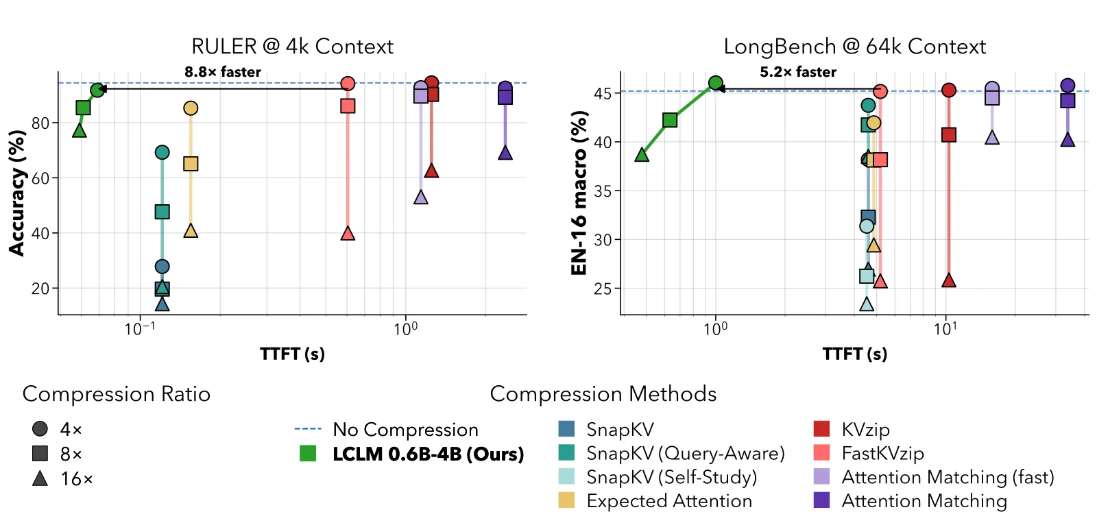
Strategy three: compress the context before the model sees it. End-to-End Context Compression (LCLM) moves the savings upstream: a 0.6B encoder pools blocks of input into single soft tokens at 1:4, 1:8, or 1:16 compression, and a 4B decoder reads the latents instead of the full sequence. The decoder never encodes the whole document, so prefill time and cache both shrink by the ratio.

Key numbers

Measurement	Gemini 1.5 (giant window)	FlashMemory-DeepSeek-V4 (sparse KV)	LCLM (latent compression)	Source
Demonstrated context	>99% retrieval recall up to at least 10M tokens	Evaluated at 500K tokens (beyond-500K is open)	Tested toward 512K to 1M tokens	papers above
Memory effect	None; full window stays resident	KV cache at 13.5% of full baseline (~7x); >90% of KV overhead suppressed at 500K	4x/8x/16x fewer input tokens; peak memory plateaus as context grows	papers above
Accuracy cost	Recall benchmarked >99%; deep multi-hop reasoning over the whole window is not what the benchmark measures	+0.6% absolute on average across LongBench-v2, LongMemEval, RULER	1:4 nearly lossless vs. the uncompressed 4B decoder; 1:16 shows a measurable gap on exact recall	papers above
Extra training	Frontier-scale pretraining of an MoE model; Pro matches 1.0 Ultra at lower serving cost	Indexer only, trained as a standard dual-encoder with the backbone never loaded	Joint 0.6B encoder + 4B decoder trained on ~350B tokens across four stages	papers above
Retrieval escape hatch	The window is the retrieval surface	Lookahead prediction pulls quiet chunks back before they are needed	EXPAND(i) returns the original 512-token chunk, buying back needle exact-match	papers above

Read the table with one rule in mind: these are three different machines measured on three different tracks. Gemini 1.5’s >99% is needle-style recall recall on a model built for it; FlashMemory’s +0.6% is a sparsification delta against its own dense baseline; LCLM’s lossless claim is relative to a 4B model, not to a frontier one. Same-harness comparisons do not exist across the rows.

Where each one spends its money

The giant window spends it everywhere, evenly. Attention over 10M tokens is quadratic in the worst case, so Gemini 1.5 pairs the window with mixture-of-experts efficiency so that the per-token compute stays sane, and the report’s cost claim is that 1.5 Pro matches or beats the previous 1.0 Ultra flagship while being cheaper to serve. The economics work because Google amortizes the pretraining; a team serving its own model this way pays the full frontier bill. And the window being huge does not make reasoning huge: locating one fact across 10M tokens is a solved benchmark shape, synthesizing scattered evidence across all of it is not measured by the retrieval suite. The Kalamang result, learning to translate a language with fewer than 200 speakers from one grammar book placed in context, is the more durable demonstration of what the window is actually for: in-context skill acquisition, not search.

Sparse KV spends it on a second model to serve. FlashMemory’s indexer is a real component: it adds latency, it adds a dual-encoder to deploy alongside the backbone, and its quality is the whole game. A mispredicted chunk is a chunk that holds the answer and is no longer in memory. The +0.6% average across LongBench-v2, LongMemEval, and RULER is the reassuring version of that story, but an average hides catastrophic single misses on needle queries, which is exactly where “was the chunk I dropped the chunk with the answer?” stops being an edge case. The compensating design choice is lookahead: instead of keeping what was attended in the past, the indexer anticipates the next span, so a chunk that goes quiet for thousands of tokens and then becomes critical can be pulled back before it is needed.

Latent compression spends it on training, then saves on every request. LCLM’s 350B-token four-stage recipe (adapter warmup, encoder training, end-to-end continual pre-training, supervised fine-tuning) is the price of moving compression from an inference-time heuristic into a trained component. The payoff is structural: KV-cache eviction methods like SnapKV or KVzip compress after the model has already paid to encode the tokens, so their compression time is roughly fixed; LCLM compression gets faster as the ratio rises, because there are fewer soft tokens to produce. And at high compression, LCLM’s peak memory plateaus as context grows, while an Attention Matching baseline runs out of memory near 512K to 1M tokens on the same hardware. The catch: the encoder window is W=1024, so very long inputs cross window boundaries and information spanning a boundary gets split; and the decoder still pays for the latents it reads, which caps how far encoder-side savings carry at extreme length.

When to use which

• You control the model, the budget, and the product surface, and want the simplest architecture: the giant window. Gemini 1.5 shows the window itself can be the retrieval system, at frontier-pretraining cost.
• You already serve an existing frontier model and 500K-token requests are running out of GPU memory: sparse KV selection. FlashMemory’s 13.5% average cache with accuracy flat to +0.6% is the least invasive fix, and its decoupled dual-encoder training means a small team can actually do it.
• Prefill cost and time-to-first-token dominate, you can train, and 4B-class quality is enough: latent compression. LCLM at 1:4 is close to free; at 1:16 it is a deliberate trade of exact recall for memory. The EXPAND tool is the practical bridge: compressed-by-default context, original chunks on demand.
• Your task needs exact recall over very long documents and none of the above apply: none of these replaces a retrieval pipeline. All three papers implicitly concede this: Gemini 1.5 by benchmarking needle recall rather than multi-hop synthesis, FlashMemory by pulling chunks back on prediction, LCLM by adding EXPAND.

Limits and open questions

The honest gap is that no controlled experiment compares these strategies head-to-head on one model, one benchmark suite, one hardware budget. FlashMemory’s numbers are deltas against its own dense DeepSeek-V4 baseline; LCLM’s are against an uncompressed 4B decoder; Gemini 1.5’s are a capability report with no compression arm at all. The LCLM models are 0.6B and 4B, so whether joint compression training transfers to frontier-scale decoders or past 1:16 is unshown. FlashMemory is tied to one backbone, and how LSA ports to other architectures, or beyond 500K, is open. And “the window is 10M tokens” continues to mean “retrieval works to 10M tokens,” which is a weaker claim than “the model reasons over 10M tokens.” For the mechanics these approaches compete with, namely KV cache quantization, head-specialization sparsity, and plain sparse attention, see KV Cache Compression Explained and Sparse Attention vs Full Attention.

FAQ

What are the three ways to handle a million tokens of context?

Scale the native window (Gemini 1.5, >99% recall to at least 10M tokens), sparsify the KV cache at decode time (FlashMemory-DeepSeek-V4, 13.5% of full cache at 500K tokens), or compress the context into soft tokens before the model reads it (LCLM, 1:4 to 1:16 compression with a 0.6B encoder and 4B decoder).

Which long-context approach loses the least accuracy?

On the numbers each paper reports: FlashMemory is flat to +0.6% average across LongBench-v2, LongMemEval, and RULER, and LCLM at 1:4 is nearly lossless against its uncompressed 4B decoder. LCLM at 1:16 shows a measurable gap on exact-recall tasks. But these are different models on different harnesses, so “least” cannot be answered with a single cross-paper number.

Does a 10M-token context window make RAG obsolete?

No. Gemini 1.5’s own report benchmarks needle-style retrieval recall, not deep synthesis across the whole window, and long prompts stay expensive and latency-heavy. FlashMemory and LCLM both end up reintroducing retrieval-shaped machinery (lookahead chunk prefetching and the EXPAND tool), which is the field conceding that search and context solve different problems.

What is the cheapest way to serve 500K tokens of context?

If the model already exists: FlashMemory-style sparse KV, because the indexer trains as a standalone dual-encoder without loading the backbone and cuts resident cache to 13.5% on average. If you can train a smaller system from scratch: LCLM-style compression, whose memory plateaus at long context where eviction-based baselines run out of memory near 512K to 1M tokens.

Why does LCLM compression get faster at higher ratios while KV-cache methods do not?

KV-cache eviction (SnapKV, KVzip) runs after the model has encoded every token, so its compression cost is roughly fixed whatever ratio you pick. LCLM compresses before the decoder, in the encoder, so a 1:16 ratio produces four times fewer soft tokens than 1:4, and fewer tokens to produce means less compression work.