
Interpretability · Language Models
Sparse Autoencoders Explained: From Superposition to Readable Features
LLM neurons are polysemantic: one cell fires for French text, DNA and HTTP at once. A sparse autoencoder unpacks that superposition into single-meaning features, and GemmaScope scaled it to 400+ open SAEs.
How it works
The unit of computation inside a language model is not the neuron. A single neuron typically fires for many unrelated concepts at once; one famous example lights up for French text, DNA sequences and HTTP requests. The leading explanation is superposition: a model with d neurons wants to represent far more than d features, so it packs features into overlapping, non-orthogonal directions and tolerates a little interference. If that is true, reading neurons one by one is the wrong move, and the real units are sparse features living in an overcomplete basis with more directions than neurons.
The Anthropic sparse autoencoder paper (“Towards Monosemanticity”) is the compact demonstration that this bet pays off. An SAE is deliberately simple: one hidden layer wider than the model dimension, trained only to reconstruct the activation vector while an L1 penalty forces the hidden code to be mostly zero. The decoder’s columns become a learned dictionary of feature directions. Because almost all entries are zero for any given token, each surviving entry is forced to carry one specific, reusable meaning: concepts like an apostrophe-context feature or a closing-parenthesis feature that you can name in a few words. Nobody labels features in advance; the interpretable structure is discovered, not imposed. Classic dictionary learning, applied to transformer activations instead of image patches.
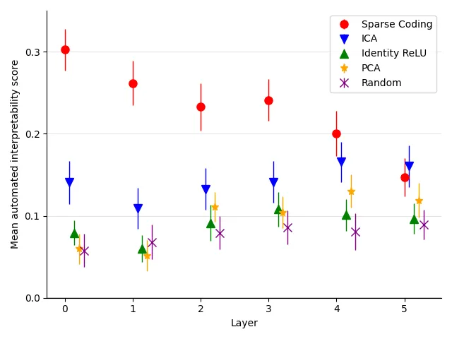
The paper’s evidence has two legs. First, under both blind human raters and an automated GPT-based scoring protocol, SAE features are rated more interpretable than the model’s own neurons, PCA/ICA components, and the raw residual-stream basis. Second, the features are causal, not just correlational: on the indirect-object-identification task the authors localize the specific features responsible for the counterfactual behavior, at a finer granularity than any prior decomposition, and editing those features moves the output in the predicted direction.
GemmaScope is what happened when an industry lab scaled the same recipe until it stopped being cheap. DeepMind trained more than 400 JumpReLU SAEs on every layer and sub-layer of Gemma 2 2B and 9B, plus select layers of 27B: for each transformer block there are three sites (attention-head outputs before the final projection, MLP outputs, and the post-MLP residual stream), spanning all 26 layers of 2B and all 42 layers of 9B. Dictionaries range from 2^14 (about 16K) up to 2^20 (about 1M) latents, each SAE trained on 4–16B tokens. The release (over 2,000 checkpoints and 30M+ features, weights on Hugging Face with a feature browser on Neuronpedia) exists because training that suite yourself was the cost wall: DeepMind spent over 20% of GPT-3’s training compute and saved roughly 20 PiB of activations to produce it.
Two design choices in GemmaScope are worth understanding, because they are where the field currently disagrees with itself. The activation function is JumpReLU: a learnable per-feature threshold, so a feature fires only when its pre-activation clears its own bar and the number of active features varies by token, unlike TopK, which forces exactly k active features everywhere. DeepMind reports a slight Pareto improvement over Gated and TopK SAEs on the reconstruction-versus-sparsity frontier, with the honest footnote that on human-rated interpretability the three families were nearly indistinguishable: the win is on the fidelity metric, not on readability. And there is no single “correct” dictionary size. Widening from 2^14 to 2^19 latents reliably lowers delta loss (the extra cross-entropy from splicing the SAE into the model) at fixed sparsity, but with diminishing returns and no guarantee the extra capacity learns genuinely new features rather than recombining old ones.
Key numbers
The two papers answer different questions (one proves the method, the other maps its scale), so their numbers are not a same-harness benchmark comparison. Treat the table as a lineage, not a leaderboard.
| Milestone | Model probed | What is decomposed | Dictionary width | Headline figures | Source |
|---|---|---|---|---|---|
| Anthropic SAE (2023) | small transformer LMs | residual-stream activations | overcomplete, wider than model width (exact size not the point) | autointerpretability beats neurons, PCA/ICA and residual basis; IOI circuit localized causally at finer granularity than prior work | paper page |
| GemmaScope (2024) | Gemma 2 2B and 9B, select 27B layers | 3 sites per block × 26 layers (2B) / 42 layers (9B) | 2^14 to 2^20 latents, i.e. ~16K to ~1M | 400+ SAEs, 2,000+ checkpoints, 30M+ features, 4–16B tokens per SAE, >20% of GPT-3 compute, ~20 PiB of saved activations | paper page |
Not directly comparable: the Anthropic numbers are qualitative scoring results, the GemmaScope numbers are coverage and training-cost figures. No shared metric or harness exists between them.
Within GemmaScope’s own results, three measured patterns matter more than any single figure:
- Site matters more than width. Residual-stream SAEs consistently show the highest delta loss (small reconstruction errors there hurt downstream predictions the most), while attention and MLP sites are easier to fit.
- Base models transfer to chat. SAEs trained only on base Gemma 2 9B reconstruct instruction-tuned 9B activations almost as well as SAEs trained on the IT model directly, so you do not necessarily need a separate SAE per model variant.
- English-heavy training shows. Delta loss is lowest on math data and highest on multilingual text (Europarl), mirroring the pretraining mix.
What SAEs are for
Feature dictionaries are instruments, not decorations. With a trained SAE you can amplify or suppress a specific feature and watch the model’s behavior change: the mechanism behind the “Golden Gate Bridge” demos where a model amplified on one feature would not stop talking about it. That turns interpretability from a post-hoc story into an intervention with a knob, which is the property that makes SAEs the default first tool for opening up a language model. Within roughly a year of the Anthropic paper, frontier labs had scaled the recipe to production models, and GemmaScope removed the remaining cost wall for everyone else: a researcher can now load an SAE for layer 20 of Gemma 2 9B and start reading features without owning a GPU cluster.
Limits and open questions
The encouraging version and the honest version of this story differ. Interpretability is measured, not guaranteed: “more interpretable than a neuron” is a low bar, and plenty of features remain murky under both human and automated scoring. The L1 sparsity penalty leaves dead and duplicated features, and choosing dictionary width and penalty weight is still partly art; later work spent significant effort on exactly these failure modes. Reconstruction is lossy, so an SAE is a lens on the model, not a faithful rewrite of it; whatever it drops is invisible to your analysis. GemmaScope’s own candid caveat is that there is still no consensus metric for whether an SAE is “good”: delta loss and fraction-of-variance-unexplained measure reconstruction, not interpretability, and the two can diverge. Feature splitting is unresolved: wider dictionaries sometimes learn genuinely new features, sometimes just recombine existing ones, with no clean way to tell which. And SAEs systematically miss features that only appear in wider dictionaries, meaning no single SAE gives a complete picture. The safest takeaway for practitioners: treat reported numbers as evidence for the paper’s setting, choose the site and width for your budget, and validate the specific features you intend to steer.
FAQ
What is a sparse autoencoder (SAE) in LLM interpretability?
A sparse autoencoder is a one-hidden-layer network trained to reconstruct a language model’s internal activations while an L1 penalty forces the hidden code to be mostly zero. Its decoder columns form a dictionary of feature directions, each of which tends to fire for a single human-nameable concept, unpacking the polysemantic “superposition” of neurons into readable units.
How do sparse autoencoders find interpretable features where neurons fail?
Neurons are polysemantic because the model packs more features than it has neurons into overlapping directions. The SAE’s hidden layer is deliberately overcomplete (wider than the model dimension), and the sparsity penalty means only a few entries are active per token, so each active entry must carry one specific meaning. The interpretability is discovered through reconstruction plus sparsity, with no human labeling.
What is GemmaScope and how many features does it cover?
GemmaScope is DeepMind’s open suite of more than 400 JumpReLU SAEs trained on every layer and sub-layer of Gemma 2 2B and 9B plus select 27B layers, released as 2,000+ checkpoints covering 30M+ learned features. Training it took over 20% of GPT-3’s compute and roughly 20 PiB of saved activations; the weights are free on Hugging Face.
What is the difference between JumpReLU and TopK sparse autoencoders?
TopK forces exactly k features to be active on every token, while JumpReLU gives each feature its own learnable threshold so the active count varies by token. In GemmaScope, JumpReLU sits slightly higher on the reconstruction-versus-sparsity frontier than Gated and TopK, but human raters found the three families nearly indistinguishable in interpretability.
Are sparse autoencoders better than reading neurons directly?
On the evidence in these papers, yes for finding single-meaning units: SAE features score higher than neurons, PCA/ICA components, and the residual basis under both blind human and automated scoring, and at least one circuit (indirect object identification) was localized causally at finer granularity. But an SAE is a lossy lens: reconstruction errors mean it is a view of the model, not a complete transcription of it.